Market Regime Detection: From Hidden Markov Models to Wasserstein Clustering

Financial markets move through distinct phases — bullish rallies, sharp crashes, quiet consolidations, and volatile swings. These market regimes differ not just in price direction, but in their underlying statistical properties: volatility, correlation structure, and risk behavior.

Detecting when markets transition between regimes can dramatically improve trading strategies, risk management, and model retraining for quantitative funds.

Traditionally, regime detection has relied on Hidden Markov Models (HMMs). But newer approaches — particularly those based on Wasserstein distance from optimal transport theory — offer a more robust, data-driven alternative.

Let’s explore both approaches with theory and hands-on code.

Part 1: Hidden Markov Models for Regime Detection

The Concept

An HMM assumes the market exists in some hidden state at any given time (like “bull” or “bear”) that we cannot observe directly. Instead, we observe returns whose statistics depend on that hidden state.

Formal Setup:
— Hidden state: zₜ ∈ {1, 2, …, K}

— Observed return: rₜ ∼ 𝒩(μ_zₜ, σ_zₜ²)

— State transitions follow a Markov chain: P(zₜ = j | zₜ₋₁ = i) = Aᵢⱼ

where A is the state transition matrix.

The model learns:
1. The number of regimes K

2. Each regime’s distribution (μₖ, σₖ)

3. Transition probabilities between regimes Aᵢⱼ

Python Implementation

import numpy as np  
import pandas as pd  
import yfinance as yf  
from hmmlearn.hmm import GaussianHMM  
import matplotlib.pyplot as plt  
  
# Download S&P; 500 data  
data = yf.download('SPY', start='2015-01-01', end='2025-01-01')  
returns = np.log(data['Close'] / data['Close'].shift(1)).dropna()  
  
# Fit a 2-state HMM  
model = GaussianHMM(n_components=2, covariance_type="full", n_iter=200, random_state=42)  
model.fit(returns.values.reshape(-1, 1))  
  
# Predict hidden states  
states = model.predict(returns.values.reshape(-1, 1))  
  
# Visualize  
plt.figure(figsize=(12, 6))  
for state in range(2):  
    mask = (states == state)  
    plt.plot(returns.index[mask], data['Close'].loc[returns.index[mask]],   
             '.', markersize=4, label=f'Regime {state}')  
plt.legend()  
plt.title('HMM-Based Market Regime Detection')  
plt.ylabel('SPY Price')  
plt.show()  
  
# Print regime characteristics  
for state in range(2):  
    regime_returns = returns.values[states == state]  
    print(f"Regime {state}: Mean={regime_returns.mean():.4f}, Std={regime_returns.std():.4f}")

What Happens:
— The HMM typically identifies two regimes: low-volatility (steady growth) and high-volatility (crisis periods)
— One regime corresponds to normal bull markets, the other to bear markets or crashes

Limitations of HMMs

1. Assumes Gaussian returns — unrealistic during market crashes and tail events
2. Markovian assumption — future state depends only on current state, ignoring longer history
3. Sensitive to initialization — different starting points can yield different results
4. Parametric — you impose distributional structure rather than discovering it from data

This motivates a more flexible approach: Wasserstein-based clustering.

Part 2: Wasserstein Distance for Regime Detection

The Core Idea

Instead of assuming parametric distributions, we treat each time window of returns as an empirical distribution and cluster these distributions based on their geometric differences.

Step-by-Step Approach

1. Segment returns into windows
   — Example: 20-day rolling windows with 10-day steps
   — Each window = one “market snapshot”
2. Represent each window as a distribution
   — Each window’s empirical distribution of returns
3. Compute distances using Wasserstein distance
   — The Wasserstein distance measures the minimum “cost” to transform one distribution into another
   — For 1D distributions: W₁(μ, ν) = ∫₀¹ |F_μ⁻¹(t) − F_ν⁻¹(t)| dt
   — where F⁻¹ is the quantile function (inverse CDF)
4. Cluster using modified k-means
   — Replace Euclidean distance with Wasserstein distance
   — Replace arithmetic mean with Wasserstein barycenter

This discovers regimes directly from the data with no parametric assumptions.

Why Wasserstein?

• Sensitive to distributional shape , not just moments (mean/variance)
• Handles non-Gaussian returns naturally, including fat tails and jumps
• Robust to noise without requiring distribution assumptions
• Provides interpretable distances between market states

Python Implementation

import numpy as np  
import pandas as pd  
import yfinance as yf  
from scipy.stats import wasserstein_distance  
from sklearn.manifold import MDS  
from sklearn.cluster import KMeans  
import matplotlib.pyplot as plt  
  
# Download data  
data = yf.download('SPY', start='2015-01-01', end='2025-01-01')  
returns = np.log(data['Close'] / data['Close'].shift(1)).dropna().values  
  
# Create rolling windows  
window_size = 20  
step_size = 10  
segments = []  
segment_dates = []  
  
for i in range(0, len(returns) - window_size, step_size):  
    segments.append(returns[i:i + window_size])  
    # Store the end date of each window for plotting  
    segment_dates.append(data.index[i + window_size])  
  
# Compute Wasserstein distance matrix  
n_segments = len(segments)  
distance_matrix = np.zeros((n_segments, n_segments))  
  
for i in range(n_segments):  
    for j in range(i + 1, n_segments):  
        dist = wasserstein_distance(segments[i], segments[j])  
        distance_matrix[i, j] = dist  
        distance_matrix[j, i] = dist  
  
# Embed into 2D space using MDS (to visualize)  
mds = MDS(n_components=2, dissimilarity='precomputed', random_state=42)  
embedding = mds.fit_transform(distance_matrix)  
  
# Cluster in embedded space  
n_clusters = 2  
kmeans = KMeans(n_clusters=n_clusters, random_state=42)  
labels = kmeans.fit_predict(embedding)  
  
# Visualize clusters  
plt.figure(figsize=(12, 6))  
colors = ['blue', 'red', 'green', 'orange']  
  
for cluster in range(n_clusters):  
    cluster_mask = (labels == cluster)  
    cluster_dates = [segment_dates[i] for i in range(len(segment_dates)) if cluster_mask[i]]  
    cluster_prices = data['Close'].loc[cluster_dates]  
    plt.scatter(cluster_dates, cluster_prices,   
                c=colors[cluster], s=10, alpha=0.6, label=f'Regime {cluster}')  
  
plt.legend()  
plt.title('Market Regime Detection using Wasserstein Distance')  
plt.ylabel('SPY Price')  
plt.xlabel('Date')  
plt.xticks(rotation=45)  
plt.tight_layout()  
plt.show()  
  
# Print cluster statistics  
for cluster in range(n_clusters):  
    cluster_segments = [segments[i] for i in range(len(segments)) if labels[i] == cluster]  
    all_returns = np.concatenate(cluster_segments)  
    print(f"Regime {cluster}: Mean={all_returns.mean():.4f}, Std={all_returns.std():.4f}, "  
          f"Count={len(cluster_segments)} windows")

Interpretation

• The algorithm automatically identifies distinct regimes without any distributional assumptions
• High-volatility periods (like the 2020 crash) typically form one cluster
• Calm, steady growth periods form another cluster
• The method captures true distributional shifts, not just changes in mean/variance

Conceptual Comparison

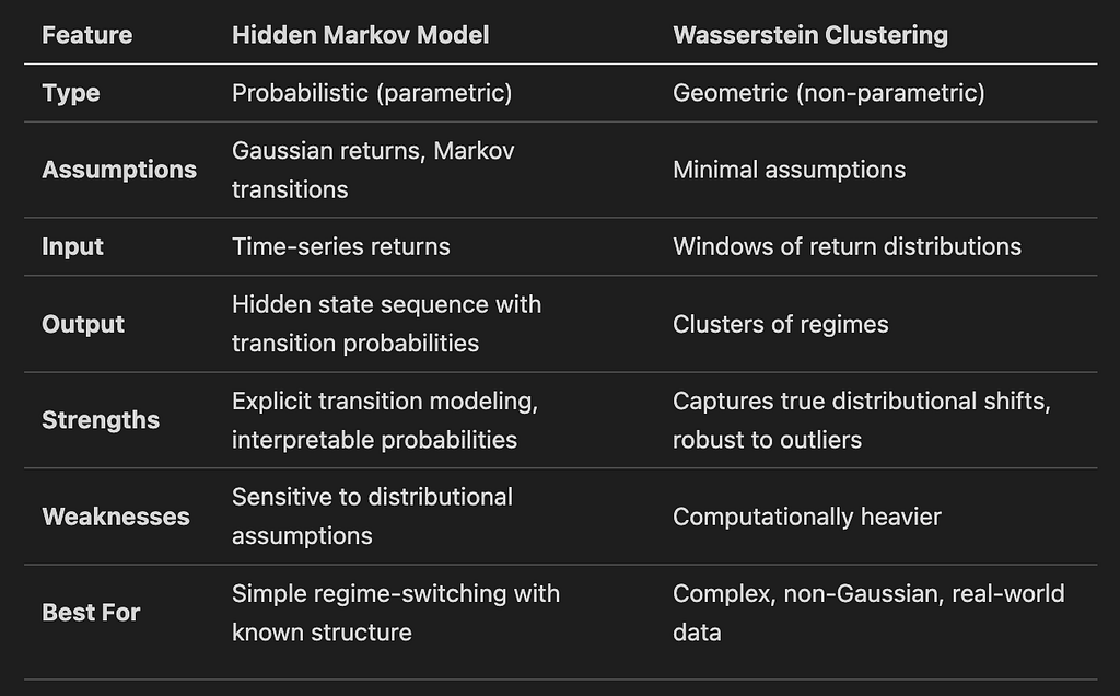
Practical Recommendations

Use HMMs when:
— You have small datasets
— You want explicit transition probabilities
— Your returns are approximately Gaussian
— Interpretability is crucial

Use Wasserstein clustering when:
— Markets exhibit heavy tails or jumps
— You want to discover regimes without assumptions
— Data is noisy or non-stationary
— Distributional differences matter more than just mean shifts

Hybrid approach:
— Use Wasserstein clustering to identify regimes
— Train separate models (HMM or ML models) within each regime
— Combine the strengths of both methods

Key Takeaways

1. Market regimes are statistical behaviors , not just price trends
2. HMMs model regimes explicitly but rely on strong distributional assumptions
3. Wasserstein methods discover regimes from data with minimal assumptions
4. In practice , Wasserstein k-means provides robust, unsupervised regime classification for both research and live trading
5. Both methods are complementary and can be combined for better results

References

• Horvath, B., Issa, Z., & Muguruza, A. (2021). Clustering Market Regimes Using the Wasserstein Distance. arXiv:2110.11848. [Also published in Journal of Computational Finance, 28(1), 1–39, 2024]
• Hamilton, J. D. (1989). A New Approach to the Economic Analysis of Nonstationary Time Series and the Business Cycle. Econometrica, 57(2), 357–384.
• Peyré, G., & Cuturi, M. (2019). Computational Optimal Transport. Foundations and Trends in Machine Learning, 11(5–6), 355–607.

Jupyter Notebook: <https://gist.github.com/arshadansari27/5ca607d8c695784da737965fe536a95b>

---

Market Regime Detection: From Hidden Markov Models to Wasserstein Clustering was originally published in Hikmah Techstack on Medium, where people are continuing the conversation by highlighting and responding to this story.